

My boss, Joe DeFranco, has always voiced his opinion on how variations of heavy sled sprint training can result in greater sprint performances, specifically with American football clients. I started out as a high school football client at DeFranco’s Training Systems in 2008, at the age of 17. At that time, we had a small facility with no access to any field space outside of the asphalt in the parking lot.
Joe had to get creative—and creative usually meant many variations of heavy sled runs. Sled pushes, sled sprints, sled drags… you name it! Joe always had a stopwatch around his neck and timed every repetition. No matter what resistance was on the sled, we had to give it our best effort and aim for the best time.
Even though we had no field space to run sprints, we all noticed that this heavy sled training was making us faster. Our ability to accelerate seemed to be drastically improving. However, due to the lack of field space, it was hard to determine if it was actually helping our sprint performance or not. Feeling a certain way is one thing, but what would the measurements and data show?
DeFranco’s gym then moved to a new location, with access to a 30-yard strip of turf. It wasn’t the best distance available for sprint training, but we could at least work on starts and 10-yard runs unloaded. Now, with the help of fully automatic timing (FAT), Joe could measure unloaded 10-yard runs and see if the heavy sled training was actually doing anything for performance gains. What Joe found was that 10-yard sprint times were improving after cycles of heavy sled training. In a sport where so much is measured by the ability to get off the ball, this appeared to have some important implications for American football players.
Horizontal Force Production
Recently, the works of JB Morin, Matt Cross, Pierre Samozino, Matt Brughelli, Scott Brown, and many others have attempted to make the historical concept of improving sprint performance with heavy sled running more accessible, and easier to understand and measure. One of the interesting concepts that I read from the researchers listed above was how elite level sprinters are able to produce more net horizontal force at higher velocities than lower level sprinters.
It’s important to explain what is meant by “net horizontal force.” With every stride, a sprinter produces force onto the ground that can be split into a vertical and a horizontal component in the sagittal plane of motion. The combination of vertical and horizontal forces in the sagittal plane is known as the resultant force, or simply the force that results from this combination. The net horizontal force describes the force being generated to propel the body horizontally. When running, ground contacts with more net horizontal force production will result in greater propulsion in the sagittal plane. Ground contacts with less net horizontal force production can result in inefficient braking forces from vertical influence. For anyone trying to sprint from point A to point B, net horizontal force production is certainly your friend.
As an athlete sprints, he/she will attempt to propel forward by putting force into the ground and producing net horizontal force and impulse, which is the force multiplied by the duration of the ground contact. However, as the athlete reaches maximum velocity, the net horizontal force production will inevitably drop and vertical forces will predominate in magnitude, notably because athletes must work against gravity, which is vertically oriented. As mentioned before, the best sprinters are able to prolong this inevitable drop and continue to produce higher ratios of force (net horizontal to resultant force) at faster and faster speeds. So, the question then becomes: If less-efficient athletes produce high ratios of net vertical force, how can we expose them to longer durations of net horizontal force production? For JB Morin and his colleagues, the answer may be found with heavy sled sprinting and trying to find an “optimal” sled load with which athletes and sprinters maximize their power and net horizontal force ratios in the sprinting motion.
Optimal Loading for Maximizing Power
A paper led by Matt Cross on “Optimal Loading for Maximizing Power During Sled-Resisted Sprinting” [1] was published in 2016 and took the sports performance world by storm. Traditionally, sled-resisted sprinting recommendations were such that no more than 10% of an athlete’s body weight should be on a sled or that no more than a 10% drop in velocity or split time should occur. However, in this paper, Cross and his colleagues recommended that, to achieve maximum power, movement velocity would have to be slowed down to 48-52% max velocity and sled loads should be in the range of 69-91% body weight for mixed-sport athletes and 70-96% body weight for sprinters! Surely that’s insanity, right?
Well, before we call these guys nuts, let’s consider what they are reportedly measuring and what these measurements mean. Below is a list of measurements that can be used to better quantify sprint performance. I give my best attempt to provide their definitions and a simplistic explanation of what they mean [2]:
V0 (m/s):
- Theoretical maximal running velocity if mechanical resistances against movement were to become nothing, or 0. This is slightly higher than the actual maximum velocity of the athlete.
- Basically, this describes the highest potential speed of the athlete and can be used to determine training loads as a percentage of max velocity.
F0 (N/kg):
- Theoretical maximal horizontal force production per unit of body mass. This corresponds to the initial push of the athlete into the ground during acceleration.
- Higher values indicate more horizontal force production.
Pmax (W/kg):
- Maximum horizontal power capability, per unit of body mass, during sprint acceleration. This is the theoretical optimal combination of force and velocity, and can be graphically depicted as the apex of the power-velocity second-degree polynomial relationship (think of the highest point on a graph of a power curve).
- Ultimately, this is the goal of optimizing sprint training. Once the relationship between force and velocity is balanced for an individual, the aim then becomes producing as much horizontal power as possible.
Fopt (N/kg):
- The theoretical optimum force production to elicit maximum horizontal power. This is considered against the theoretical optimum velocity.
- This is how much force is necessary to optimize and maximize horizontal power output.
Vopt (m/s):
- The theoretical optimum velocity achieved to elicit maximum horizontal power. This is considered against the theoretical optimum force.
- This is how much running velocity is necessary to optimize and maximize horizontal power output. If an athlete produces his/her best efforts against a resistance that “forces” him/her to run at Vopt, then the power output will be maximal.
Lopt (kg):
- The theoretical optimum load (sled load) necessary to elicit maximum horizontal power.
- This is where it becomes important to test and train on the same type of surface so that friction forces do not interfere with accurate calculations. For example, a 150-lb sled on field turf may slide more easily than the same load on a rubber track surface.
RF (%):
- Ratio of force. This basically describes how much of the total resultant force applied onto the ground will result in net horizontal force production.
- Athletes who efficiently apply force so that higher net horizontal forces occur will have a higher value than those who produce higher ratios of vertical force. All things being equal, the higher this ratio, the more horizontally oriented the resultant ground reaction force, and the more effective the propulsion.
DRF:
- The rate of decrease in ratio of force as speed increases linearly with increasing velocity during sprint acceleration. It’s inevitable that net horizontal force will diminish as max velocity is reached, and this value can determine the athlete’s ability to maintain net horizontal force production as speed increases.
- For example, Athlete A attains a value of 0.10 and Athlete B attains a value of 0.05. This means Athlete A will lose approximately 10% of net horizontal force with every 1 m/s increase in velocity, whereas Athlete B will only lose 5% of net horizontal force. Thus, Athlete B has more effective force application during acceleration.
- Note that this range of values is the range separating world-class sprinters from recreational runners.
So, according to this research, it seems that improving acceleration is heavily dependent upon finding the optimal combination of horizontal force and velocity (maximum horizontal power), improving the ratio of force production in the horizontal direction (avoiding unnecessary vertical force production), and maintaining horizontal force application for as long as possible as movement velocity increases with every step. It should be mentioned that during an unloaded sprint, maximal power is usually reached within one second, and the rest of the sprint acceleration puts the athlete at running velocities way beyond the optimal velocity (Vopt).
Sleds are a “no-brainer” for overloading the horizontal plane and improving horizontal force capabilities. Sprinting with a sled is also arguably the most specific strength training exercise that a sprinting athlete can do. Therefore, finding the individualized load for max power (the Lopt) would put the athlete in the best position to improve maximum horizontal power and the high sled loads could also lead to improvements in RF and lowering the percentage of DRF. It just so happened that the research from Cross et al. (2016) found the Lopt to occur anywhere between 69-96% of body mass!
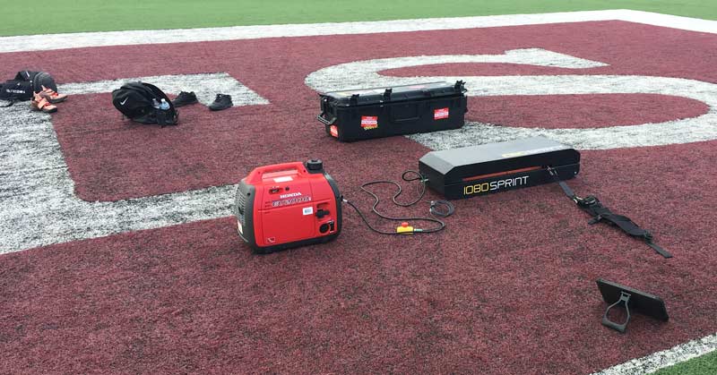
Sleds are a “no-brainer” to overload the horizontal plane and improve horizontal force. Share on XI thought back on how Joe DeFranco found improvements in sprint performance using very heavy sleds in training. Was he improving upon the aforementioned measurements of efficient force production and aiding in the maximization of horizontal power without fully realizing it? Joe had only tested unloaded 10-yard sprints and longer sprints during times of combine/pro day training with potential NFL athletes, due to the space limitations of our old facility. Luckily for us, our current location has an entire football field and track directly across the street—a perfect location for sprint work of any distance. I also happen to have a 1080 Motion Sprint machine, which I like to call the “holy grail” of resisted sprint training devices. So, I thought to myself… Let’s give this heavy sled sprinting thing a try and see what happens!
The Case Study
At the time of this project, I had been training four NFL free agent clients: two linebackers and two running backs. I wanted to see how training at a constant distance of 20 yards against the individualized load of maximum power might affect their ability to run unloaded 20-yard and 40-yard sprints. The first step was figuring out what their unloaded sprint times were, which I tested using a FAT system. This means that the start and the finish both had to be fully automatic, with a motion sensor triggering the start and a laser triggering the finish. I wanted to eliminate human error as much as possible.
It should absolutely be noted that the most accepted margin of error between FAT and hand times (i.e., using a stopwatch) is 0.24 seconds [3]. It’s important that I elaborate on what this 0.24-second margin means. It means that if a player can run a 40-yard dash in 4.50 seconds when a coach uses a stopwatch, it’s very likely that the same exact sprint could register as 4.74 seconds on a FAT system. Therefore, it’s a safe bet to assume that the split times reported below should have 0.24 subtracted from them to get an estimate of what they might be if timed by hand.
| Player | Height | Body Weight | 10-Yard Sprint (secs) | 20-Yard Sprint (secs) | 40-Yard Sprint (secs) |
| Linebacker #1 | 6’1” | 247lbs | 1.71 | 2.90 | 5.19 |
| Linebacker #2 | 6’1” | 228lbs | 1.75 | 2.93 | 4.94 |
| Running Back #1 | 5’8” | 220lbs | 1.68 | 2.79 | 4.92 |
| Running Back #2 | 5’9” | 202lbs | 1.70 | 2.97 | 4.87 |
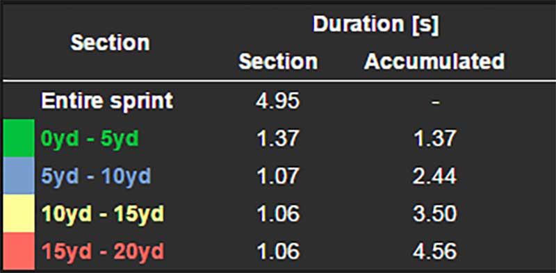
When planning the heavy sled training, I decided that I was going to follow the loading guidelines outlined in Cross et al. (2016) and then perform four weeks of training using this “optimal load” once a week. To do this, I had to find the load that corresponded to 48-52% of max velocity for each individual. I decided to base this on average velocity rather than peak velocity; the average velocity would paint a clearer picture of improvements over the entire 20-yard sprint rather than an instantaneous moment.
The absolute beauty of the 1080 Sprint machine is the amount of information that it gives you. Not only does the machine time every sprint for you using FAT, but you can see peak and average force, power, and velocity, in addition to a graphic representation of every step of that particular sprint, after every sprint performed. The resistance that the machine provides has a wide range of possibilities.
The absolute beauty of the 1080 Sprint machine is the amount of information that it gives you. Share on X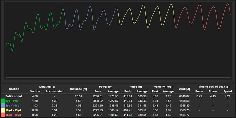
Preliminary measurements consistently showed that there is a friction coefficient on the machine of about 35% when considering field turf surface. This means that for each setting on the machine, the number should be divided by 0.35 to get a more accurate depiction of what a similar-feeling load on a regular plate-loaded sled would be. So, if we are on a turf football field and the setting on the machine is 10kg, it is likely that it would feel the same as a sled loaded with about 29kg (or 63lbs). Below is a basic table of load conversions using this friction coefficient:
| 1080 Sprint Load Setting | Approximate Equal Load on Sled |
| 3kg | 9kg (19lbs) |
| 8kg | 23kg (50lbs) |
| 15kg | 43kg (94lbs) |
| 20kg | 57kg (126lbs) |
| 25kg | 71kg (157lbs) |
| 30kg | 86kg (189lbs) |
Video 1. Sprints in gear 1 – 3kg, 8kg, 15kg
To find the maximum average velocity (V0) over 20 yards, I had each player run a 20-yard sprint against incremental load settings on the 1080 Sprint: 3kg, 8kg, 15kg, 20kg, 22kg, 24kg, 26kg, 28kg, and 30kg (the highest the machine goes). I then took the average velocity data obtained from the 1080 Sprint and plotted the numbers against the load being used at each point along an XY scatter plot in Excel. I made sure that the formula was then displayed so that I could view where the y-intercept would occur. This number would theoretically correspond to V0, as long as the coefficient of determination (R^2) was higher than 0.96. All of my guys had R^2 values of at least 0.97, so I felt confident that the velocity numbers were an accurate representation of their theoretical maximums.
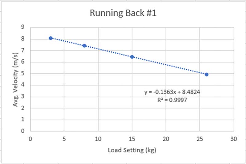
Once I had these numbers on hand, the 1080 Sprint could tell me the rest. I simply went into the testing data on the 1080 Motion Web App and found the load that corresponded to 48-52% average velocity. For example, one of my running backs had a V0 of 8.25 m/s, so I looked for the load that had him running between 3.96-4.29 m/s.
| Player | Body Weight | 1080 Sprint Setting | Adjusted for 35% Friction Coefficient | Percentage of Body Weight |
| Linebacker #1 | 112kg 247lbs | 28kg | 80kg 176lbs | 71% |
| Linebacker #2 | 104kg 228lbs | 28kg | 80kg 176lbs | 77% |
| Running Back #1 | 100kg 220lbs | 26kg | 74kg 163lbs | 74% |
| Running Back #2 | 92kg 202lbs | 26kg | 74kg 163lbs | 80% |
Since the 1080 Sprint can provide real-time feedback on every repetition, I decided that if any of the players began running faster than 52% of their estimated V0 during the session, I would adjust the load setting upwards by 2kg. This allowed me to auto-regulate the process and always ensure that the players were sprinting against the load that would put them in the 48-52% range. However, if any of the players reached the 30kg setting (the highest setting currently allowed by the 1080 Sprint machine), then they would simply just try and run faster against that load each subsequent repetition.
Training Schedule
The 1080 Sprint sessions were performed once a week. Before working with the 1080 Sprint, the athletes performed low-volume, unloaded sprint work of 10-20 yards immediately following warmups to maintain a velocity-specific stimulus to unloaded sprinting. I then had them each do four 25-yard sprints against their individual optimum load. I had them do 25 yards to ensure that 20 yards were sprinted at full effort. Lastly, I had them perform some extra sprint work against lighter loads to feel for any potentiation from the heavy loads. These lighter load sprints were performed for 25-45 yards with the intention of staying around 85-90% of unloaded split times.
| Training Session |
| Warm Up |
| 10-20yd Sprints – 3-4 reps of each |
| Optimal Load 25yd Sprints w/ 1080 Sprint – 4 total reps |
| Light Load 25yd Sprints – 2 total reps |
| Light Load 45yd Sprints – 2 total reps |
Video 2. 45 yard sprints with 1080 Sprint.
Looking at the Results
So, what happened? Well… a lot.
The first note worth mentioning is that by Week 4, three out of four of the players were using the 30kg setting, meaning they reached the highest available resistance granted by the 1080 Sprint machine. The other player, Linebacker #2, stayed at a constant load setting from Weeks 1-4 (28kg). The progression is laid out in Figure 7.
| Week 1 | Week 4 | |||
| Player | Load (Setting/0.35) | Percentage of Body Mass | Load (Setting/0.35) | Percentage of Body Mass |
| Linebacker #1 | 80kg 176lbs | 71% | 86kg 189lbs | 77% |
| Linebacker #2 | 80kg 176lbs | 77% | 80kg 176lbs | 77% |
| Running Back #1 | 74kg 163lbs | 74% | 86kg 189lbs | 86% |
| Running Back #2 | 74kg 163lbs | 80% | 86kg 189lbs | 94% |
Video 3. Sprinting with week 4 optimal load.
The paper by Cross et al. (2016) assumed that the optimal loading range would occur somewhere between 69% and 96% body mass and my data showed that all of my football players fell within this range (71-80%) in Week 1. Again, despite upwards of a 14% increase in load as seen with Running Back #2, the mean velocity stayed between 48% and 52% of V0. This indicates that the players whose loads increased over four weeks could maintain their horizontal velocity in the face of increasing resistances. They were becoming more powerful.
Of course, it’s easy to comprehend that more power was being generated, but I wanted to see how changes might have occurred with maximum velocity (V0), maximum relative horizontal force (F0), and maximum relative horizontal power (Pmax). Here are the pre-testing and post-testing numbers.
| F0 (N/kg) | V0 (m/s) | Pmax (W/kg) | ||||
| Player | Pre | Post | Pre | Post | Pre | Post |
| Linebacker #1 | 6.00 | 6.33 | 8.39 | 8.40 | 12.59 | 13.29 |
| Linebacker #2 | 6.17 | 6.77 | 8.51 | 8.50 | 13.12 | 14.40 |
| Running Back #1 | 6.87 | 6.92 | 8.48 | 8.71 | 14.57 | 15.06 |
| Running Back #2 | 7.21 | 7.28 | 8.25 | 8.59 | 14.87 | 15.64 |
All of the players improved their relative maximum power after four weeks. Both of the running backs did so through greater proportional rises in V0, while the linebackers were the opposite, seeing rises in power through greater proportional rises in F0.
I should make sure to state that this particular four-week program was not based upon individual deficiencies in force-velocity profiling. All of the athletes performed the same routine, once a week for four weeks. However, since the overall training program included a combination of unloaded sprints, sprints against load of maximum power, and lighter resisted sprints, it’s possible that everyone was able to improve upon their force-velocity deficiencies.
For example, the linebackers may have been deficient in their ability to produce net horizontal force, and based on relative force (N/kg), they both produced far less than the running backs in the pre-testing period. Their improvement in F0 may have stemmed from the heavy resisted runs. The running backs both made larger improvements in V0, which may have been a result of exposure to the light-resisted runs and unloaded runs.
One area that all players showed improvement in was the ability to accelerate at each 5-yard segment over 20 yards against their individual optimum load. During the first two weeks, most of them began decelerating between 15 and 20 yards. But by Weeks 3-4, all of them were able to continue accelerating or maintain acceleration every 5 yards. This was likely an indication of improvement in RF and DRF.
George Petrakos has referred a concept known as the Maximum Resisted Sled Load (MRSL). The MRSL is the highest load an athlete can use for a 20-meter sprint and show no deceleration at any 5-meter segment. In my case, I was measuring yardage, but from what I was seeing, it is likely that the Lopt will tend to be very close to the load corresponding to 100% MRSL as described by Petrakos. It may be possible to prescribe different training loads based on Lopt in similar ways to what Petrakos describes for loads based on MRSL.
Improvements in Sprint Times?
So, great. Everyone’s maximum horizontal power improved. Cool. But what about their sprint times? Isn’t it all meaningless if sprint times didn’t improve?
Well, let’s look at the pre- and post-testing data as it relates to split times in the 10-, 20-, and 40-yard dash. Unfortunately, one of the players (Linebacker #2) finished his time at the facility before being able to re-test his sprint times. So here is the FAT sprint time data for Linebacker #1, Running Back #1, and Running Back #2.
| 10-Yard Sprint | 20-Yard Sprint | 40-Yard Sprint | |||||
| Player | Pre | Post | Pre | Post | Pre | Post | Est. Hand Time (FAT-0.24) |
| Linebacker #1 | 1.71 | 1.65 | 2.90 | 2.75 | 5.19 | 4.86 | 4.62 |
| Running Back #1 | 1.68 | 1.58 | 2.79 | 2.68 | 4.92 | 4.68 | 4.44 |
| Running Back #2 | 1.70 | 1.68 | 2.79 | 2.75 | 4.87 | 4.77 | 4.53 |
Did sprint times improve? Yes, they did. Between these three players, a range of 0.10-0.33 seconds of improvement in FAT sprints was found after only four weeks of training. Will my findings be fully consistent with yours? Who knows, but decreases in split times at 10, 20, and 40 yards definitely occurred. It is likely that a combination of factors came together that led to these results.
Here are some considerations based on the program I did:
- Even if only 10-20 yards of distance, performing unloaded sprints at full speed after warming up allowed the players to experience sprinting against their own body mass and preserve coordination.
- Developing the ability to accelerate every 5 yards for 20 yards against horizontal resistances of 77-94% body mass likely improved each player’s RF and DRF, allowing them to produce more net horizontal force at increasing velocities and accelerating or maintaining speed throughout the entire 40-yard dash.
- Performing the light resisted sprints for upwards of 45 yards also likely played a role in improving upon DRF for each player. Having the light resistance allowed for very high efforts against relatively long distances with lower risk of CNS fatigue or potential injury.
In terms of really improving sprint performance, it would have been more optimal for me to calculate a force-velocity profile for each player and then prescribe loading parameters from there. However, my goal was to see if four weeks of sprinting against individualized loads of maximum power could improve sprint performance in NFL players and my results showed that it can, indeed.
So, there you have it. More practical evidence that sprinting against the load of maximum power (Lopt) can improve sprint performance and may be best-served as a complement to unloaded sprints and light-loaded sprints (i.e., 10-15% decrement in split time). Consider using maximum power sled sprinting as a—dare I use a pun? —powerful tool in your training tool box.
P.S. Based on my findings, 20-yard split times against Lopt were between 60% and 66% of unloaded 20-yard split times. So, although the 48-52% velocity decrement is reported by Cross et al. (2016), those numbers do not correspond to numbers based on split times. More research needs to be done to determine whether an actual normative range based solely on split times can be recommended.
Special thanks to JB Morin and Matt Cross for helping with the accuracy of the interpretation of their work.
References
- Cross, M.R., Brughelli, M., Samozino, P., Brown, S.R., Morin, J.B. (2016). Optimal Loading for Maximizing Power during Sled-Resisted Sprinting. Int J Sports Phys & Perf. 1-25.
- Morin, J.B., & Samozino, P. (2016). Interpreting power-force-velocity profiles for individualized and specific training. Int J Sports Phys & Perf. 11(2): 267-272.
- Smith, J. (2014). Applied Sprint Training. Amazon.

